Editor's note: Alexey Natekin, founder of DM Labs and chief data officer of DIGINETICA, explained the principle of gradient boosting algorithm.
Hello everyone! So far, we have covered nine topics ranging from exploratory analysis to timing analysis. Today we are going to introduce one of the most popular and practical machine learning algorithms: Gradient Boosting.
Overview
Introduction and History of Gradient Boosting
GBM algorithm
loss function
related resources
Introduction and History of Gradient Boosting
In the field of machine learning, gradient boosting is a well-known technique. Many data scientists have this technique in their toolbox because it gives great results on any given (unknown) problem.
Also, XGBoost is a common formula for ML competition champions. It was so popular that the idea of ​​stacking XGBoost became a meme. Also, gradient boosting is an important part of many recommender systems; sometimes it even becomes a brand. Let's take a look at the history and development of gradient boosting.
Gradient boosting stems from the question: Can a strong model be obtained from a large number of relatively weak, simple models? Here "weak model" refers not to a simple and basic model like a decision tree, but to a model with poor accuracy, worse than random guessing.
Mathematically, the answer to this question is yes, but it took several years to develop a practical algorithm (for example, AdaBoost), the study found. These algorithms take a greedy approach: first, a linear combination of simple models (basic algorithms) are created by reweighting the input data; second, a model (usually a decision tree) is created based on objects that were previously mispredicted (given more weight).
Many machine learning courses discuss AdaBoost, the ancestor of GBM. However, it now appears that AdaBoost is nothing more than a specific variant of GBM.
The intuition of the algorithm itself to define the weights is very clear, and it is easy to interpret through the visual method. Let's look at the toy classification problem below, where we will split the data between trees of depth 1 in each iteration of AdaBoost.
The size of the data points corresponds to their weights, which are assigned to incorrect predictions. At each iteration, we see the weights increase due to failure to classify correctly. However, if we do weighted voting, we get the correct classification:
Below is a more detailed example of AdaBoost, where we see that the weights increase as the iteration progresses, especially at the boundaries of the classification.
AdaBoost works well, but the lack of explanation as to why the algorithm is so successful is where some of the confusion arises. Some people think that AdaBoost is a super algorithm, a silver bullet, but others are sceptical and believe that AdaBoost is just overfitting.
Overfitting problems do exist, especially when the data has strong outliers. Therefore, AdaBoost's performance on this kind of problem is unstable. Fortunately, some Stanford statistics professors started working on this algorithm (these professors invented Lasso, Elastic Net, Random Forest). In 1999, Jerome Friedman popularized the lifting algorithm - Gradient Boosting (Machine), or GBM for short. This work by Friedman provides the statistical basis for many algorithms that employ the general approach of boost optimization.
Many algorithms including CART, bootstrap originate from the Stanford Statistics Department. The presentation of these algorithms leaves a place for them in future textbooks. These algorithms are very practical, and some recent work is not yet widely available. For example, glinternet.
There aren't many Friedman videos online, however, there is a very interesting interview on how CART came about and how CART solves statistical problems (much like data analysis and data science today): https://youtu.be/8hupHmBVvb0 Also recommend Hastie's lecture: https://youtu.be/zBk3PK3g-Fc, a review of data analysis by the creator of many of the methods we use every day today.
History of GBM
It took more than a decade for GBM to go from being proposed to becoming a must-have component of the data science toolbox. Extensions of GBM are used for different statistical problems: GBM model enhanced versions GLMboost, GAMboost, CoxBoost for survival curves, RankBoost and LambdaMART for ranking.
Many implementations of GBM appear on different platforms under different names: Stochastic GBM, GBDT (Gradient Boosted Decision Tree), GBRT (Gradient Boosted Regression Tree), MART (Multiple Accumulation Camp, it's hard to keep track of how popular gradient boosting has become.
At the same time, gradient boosting is heavily used for search sorting. The search ranking problem can be reformulated based on a loss function that penalizes output order errors, thus facilitating direct insertion into GBM. AltaVista was one of the first companies to introduce gradient boosting in search ranking. Soon, Yahoo, Yandex, Bing, and others also adopted this idea. Since then, gradient boosting has not only been used in research, but has become one of the core technologies in the industry.
ML competitions, especially Kaggle, have played a major role in the popularity of gradient boosting. Kaggle provides a public platform for researchers to compete on mathematical science problems with a large number of players from around the century. On Kaggle, new algorithms can be tested on real data, which gives the algorithm a chance to "shine". Kaggle provides complete information on how the model performs on different competition datasets. This is exactly what happened when gradient boosting was used in Kaggle competitions (most of the interviews with Kaggle champions since 2011 mention their use of gradient boosting). The XGBoost library quickly became popular when it appeared. XGBoost is not a novel and unique algorithm; it is just an extremely efficient implementation of the classic GBM (plus some heuristics).
The GBM experience is also the experience of many ML algorithms today: after their initial appearance, it took many years from mathematical problems and algorithmic craftsmanship to successful practical application and large-scale use.
GBM algorithm
We will solve a function approximation problem in a general supervised learning setting. The feature set is denoted as X, and the target variable is denoted as y, and we need to reconstruct the dependency of y = f(x). We reconstruct this dependency by approximating f(x) and decide which approximation is better based on the loss function L(y, f):
At this stage, we make no assumptions about the kind of f(x), the approximation model, and the distribution of the target variable. We only expect L(y, f) to be differentiable. The expression that minimizes the data loss (based on the population mean of a specific dataset) is:

Unfortunately, not only are there many such functions, but the function space has infinite dimensions. Therefore, the search space needs to be restricted to certain function families. This greatly simplifies the objective, as we now only have to solve the optimization problem of the parameter values.
There is often no simple analytical solution to finding optimal parameters, and we usually approximate the parameters iteratively. We write the empirical loss function at the beginning so that we can calculate the parameters based on the data, and write down the sum of the parameter approximations after M iterations:

Then, we just need to find an appropriate iterative algorithm that minimizes the above equation. Gradient descent is the simplest and most commonly used option. We define the gradient of the loss function over the current approximation and then subtract the gradient in the iterative calculus. In the end we just need to initialize the first approximation and choose the number of iterations M.
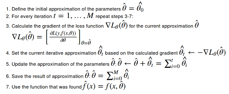
function gradient descent
Let's imagine that we can optimize in the function space, iteratively searching for the function approximation itself. We formulate the approximation as the sum of incremental improvements, each improvement as a function.
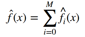
Nothing has actually happened so far; we just decided not to search for approximations as a huge model with lots of parameters (e.g. neural networks), but as a sum of functions, assuming we move in the space of functions.
To accomplish this, we need to restrict the search space to a certain family of functions:

At each step of the iteration, we need to choose the optimal parameter Ï âˆˆ â„. The problem to be solved in step t is as follows:
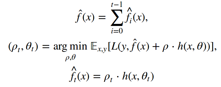
This is the key point. We define all objectives in a general form, pretending that we can define any kind of model h(x, θ) for any kind of loss function L(y, f(x, θ)). In practice, this is extremely difficult. Fortunately, there is an easy way to solve this task.
Once we know the gradient expression for the loss function, we can compute the corresponding value on the data. This way, we can train the model so that its predictions and gradients (inverse) are more correlated. In other words, we will correct the prediction based on the prediction and the least squared difference of these residuals. Therefore, step t ultimately translates to the following problem:
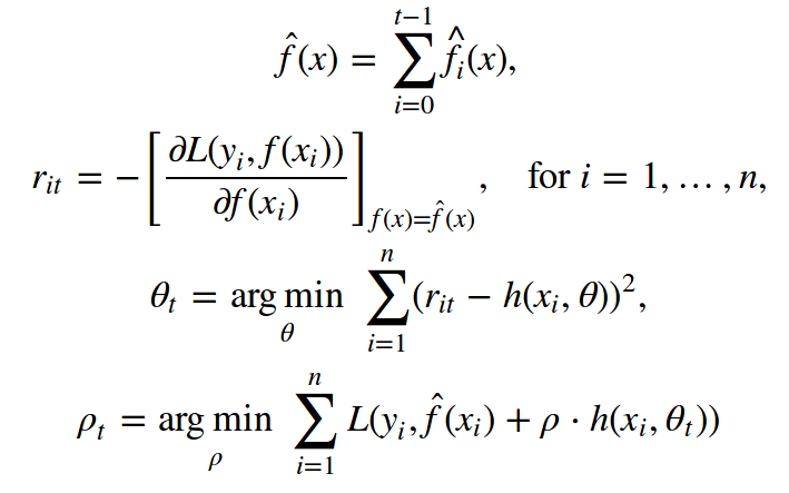
Friedman's classic GBM algorithm
Let's talk about the classic GBM algorithm proposed by Jerome Friedman in 1999. It is a supervised algorithm with the following elements:
dataset{(xi,yi)}i=1,…,n
Iteration number M
Gradient well-defined loss function L(y, f)
The function family h(x, θ) corresponding to the basic algorithm and its training process
Other hyperparameters for h(x, θ) (e.g. the depth of the decision tree)
There is still the first approximation of f0(x) left. For simplicity, a constant γ is used for the first approximation. This constant value γ and the optimal parameter Ï are both obtained by binary search or other line search algorithms based on the initial loss function (non-gradient).
The GBM algorithm process is as follows:
Initialize GBM with constant values:


Each iteration t = 1, …, M, repeat the above approximation process;
Compute pseudo-residuals rt for i = 1, …, n:

Use the regression on the pseudo residual {(xi, rit)}i=1,...,n as the basic algorithm ht(x)
Find the optimal parameter Ït according to the initial loss function of ht(x):

save

Update the current approximation:

Compose the final GBM model:

Conquer Kaggle and the world
How GBM works
Let's demonstrate how GBM works with an example. In this toy example, we need to rebuild the following function:

This is a real-valued regression problem, so we will choose the mean squared error loss function. We will generate 300 pairs of observations and then approximate them with a decision tree of depth 2. List the elements required to use GBM:
Toy data {(xi, yi)}i=1,…,300✓
Number of iterations M = 3 ✓
Mean squared error loss function L(y,f) = (yf)2✓
The gradient of L(y,f) (L2 loss) is nothing but the residual r = (yf) ✓
The basic algorithm h(x) is a decision tree ✓
Hyperparameters for decision trees: tree depth equal to 2 ✓
In terms of mean squared error, the initialization of γ and Ït is simple. When we initialize GBM, all parameters Ït are set to 1, and γ is determined according to the following formula:

We run GBM and plot two graphs: the current approximation (blue) and each tree built on the pseudo-residuals (green).
From the image above we can see that our decision tree has recovered the basic form of the function on the second iteration. However, on the first iteration the algorithm only created the "leftmost part" of the function (x ∈ [-5, -4]). This is because our decision tree does not have enough depth to create symmetric branches all at once, so it first focuses on the leftmost part with a large error.
The rest of the process is not what we expected - the pseudo-residual decreases at each step, and as the iteration progresses, the GBM gets better and better at approximating the original function. However, the construction of the decision tree determines that it cannot approximate a continuous function, which means that GBM is not very effective in this example. If you want to experiment with GBM function approximation visually, you can use the tool provided by Brilliantly wrong: http://arogozhnikov.github.io/2016/06/24/gradient_boosting_explained.html
loss function
If we wanted to solve a classification problem instead of a regression problem, what changes would be required? Just choose a suitable loss function L(y,f). It is this most important high-level opportunity that determines how we will optimize and what properties we expect the final model to have.
We didn't have to invent this ourselves - the researchers did it for us. We will now explore loss functions for the two most common objectives: regression and binary classification.
regression loss function
The most common options are:
L(y,f) = (yf)2, which is L2 loss or Gaussian loss. This classic conditional average is the simplest and most common case. If we don't have the extra information and don't require the robustness of the model, then Gaussian loss can be used.
L(y,f) = |yf|, which is L1 loss or Laplacian loss. In fact it defines the conditional median. As we know, the median is more robust to outliers, so this loss function performs better in some cases. Penalties for large deviations are not as large as L2.
Lq loss or quantile loss:

where α ∈ (0,1). Lq uses quantiles instead of medians, e.g., α = 0.75. As shown below, this function is asymmetric, penalizing observations to the right of the defined quantiles More power.
Let's experiment with the effect of Lq. The goal is to recover the conditional 75% quantile of the cosine. List the elements required for GBM:
Toy data {(xi, yi)}i=1,…,300 ✓
Number of iterations M = 3 ✓
Loss function L0.75(y,f) ✓
Gradient of L0.75(y,f)✓
The basic algorithm h(x) is a decision tree ✓
Hyperparameters for decision trees: tree depth equal to 2 ✓
The first approximation will use the desired quantile of y, but we don't know what the optimal parameter should be, so we'll use a standard line search.
The result is equivalent to the L2 loss plus a bias of about 0.135. But if we were using the 90% quantile, then we wouldn't have enough data (imbalanced classification). This needs to be kept in mind when we deal with non-standard problems.
Many loss functions have been developed for regression tasks. For example, the Huber loss function, when there are few outliers, is similar to L2, but after a defined threshold is exceeded, it is transformed to L1, thereby reducing the impact of outliers.
Below is an example with data generated from the function y = sin(x) / x, plus noise (a mixture of normal and Bernoulli distributions).
In this example, we use splines as the base algorithm. You see, gradient boosting doesn't always require using decision trees.
The above figure clearly shows the difference between L2, L1, and Huber losses. The best approximation can be obtained if we choose the optimal parameters for the Huber loss.
Unfortunately, very few of the popular libraries/packages support Huber loss; h2o does, XGBoost does not. Huber loss has to do with conditional expectations - a relatively exotic, but still worthwhile knowledge.
Classification loss function
Now let's look at the binary classification problem. It is technically possible to solve this problem based on L2 regression, but this is not the norm.
The distribution of the target variable (y ∈ {−1,1}) requires us to use the log-likelihood, so we need a different loss function. The most common choices are:
L(y,f) = log(1 + exp(−2yf)), which is logistic loss or Bernoulli loss. This loss function has an interesting property that it even penalizes correctly predicted classifications - not only optimizing the loss, but also making the classifications more spread out.
L(y,f) = exp(-yf), which is the AdaBoost loss. AdaBoost using this loss function is equivalent to GBM. Conceptually, this function is similar to logistic loss, but with a heavier exponential penalty for mispredictions.
Let's generate toy data for a new classification problem. We will use the noised cosine mentioned earlier as a basis and use the sign function to get the classification of the target variable. Our toy data is shown below (jitter noise added):
We will use logistic loss. Let's list the elements of GBM again:
Toy data {(xi, yi)}i=1,…,300, y ∈ {−1,1} ✓
Number of iterations M = 3 ✓
The loss function is logical loss, and the gradient calculation method is as follows ✓
The basic algorithm h(x) is a decision tree ✓
Hyperparameters for decision trees: tree depth equal to 2 ✓
Logistic Loss Gradient Computation
This time, the initialization of the algorithm is a little more difficult. First, our classification is not balanced (63% vs. 37%). Second, there is no known analytical formula for the initialization of the loss function, so we need to solve it by searching:
Our optimal initial approximation is around -0.273. You might have guessed that it should be a negative value, since it would be most beneficial to predict all terms as the most popular category, but there is no formula for an exact value. Now we can finally start the GBM process:
The algorithm successfully restores the separation of the classifications. You can see how the "lower part" is separated because the decision tree is more confident about correct predictions for the negative classification (-1), and you can also see how the model fits mixed classifications. Clearly, we get a large number of correctly classified observations, and some observations with large errors are due to noise in the data.
Weights
Sometimes, we come across situations where we want to use a more specific loss function. For example, on financial time series data, we may need to give greater weight to large changes in the time series; in the churn rate prediction problem, it is more useful to predict the churn rate of customers with high LTV (how much profit the customer will bring in the future) .
Statistics warriors may want to invent their own loss function, write down its gradient (including the Hessian matrix), and double-check that the function satisfies the desired properties. However, there is a high chance that an error will be made somewhere, making it computationally difficult and spending an inordinate amount of time troubleshooting.
With this in mind, a very simple approach (few people remember in practice) has been proposed: weight the observations using a weight distribution function. The simplest example is weights added to balance classification. In general, if we know that certain subsets of the data (input and target variables) are more important to our model, then we can directly assign larger weights w(x, y) to them.
The weights must meet the following conditions:
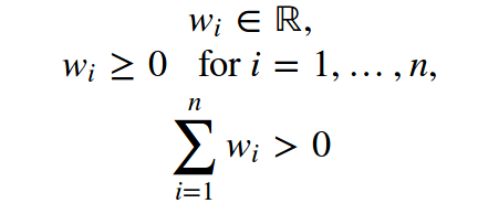
Weights can significantly reduce the time spent tuning the loss function for the current task and encourage you to experiment with the properties of the target model. Weight distribution can give full play to your creativity. For example, simply adding scalar weights:
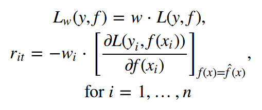
For arbitrary weights, we do not necessarily know the statistical properties of the model. Associating weights with y-values ​​often gets too complicated. For example, using a weight proportional to |y| is not equivalent in L1 loss and L2 loss (the gradient does not take into account the predicted value itself).
Now, create some very exotic weights for our toy data. We will define a brute force asymmetric weighting function:

Based on such weights, we expect to get two properties: the negative values ​​of X are less detailed, forming a function like the initial cosine. We took the GBM from the previous example, tweaked it, and ended up with:
We got the expected result. First, we can see that the pseudo-residuals on the first iteration have a large gap and look almost like the original cosine function. Second, the graph of the left half of the function is often ignored, and the function is more biased towards the half with greater weight. Third, the function from the third iteration looks similar to the original cosine function (and starts to overfit a little).
Weights are a high-risk, powerful tool that can be used to control the properties of a model. If you're going to optimize a loss function, it's worth trying the simpler problem of weighting observations first.
Epilogue
Today, we learned the theory behind gradient boosting. GBM is not a specific algorithm, but a common way to create an ensemble of models. This approach is sufficiently flexible and scalable - large numbers of models can be trained, using different loss and weighting functions.
Real-world projects and ML competitions show that on standard problems (except images, audio, very sparse data) GBM is often the most efficient algorithm (not to mention that in stacking and high-level ensembles, GBM is almost always part of it). At the same time, GBM is also used a lot in reinforcement learning (Minecraft, ICML 2016). By the way, in the field of computer vision, the Viola-Jones algorithm based on AdaBoost is still used.
In this post, we intentionally omit questions about regularization, randomness, hyperparameters of GBM. It is no accident that we have been using a very small number of iterations, M = 3. If we train GBM with 30 trees, the results will not be as predictable:
good fit
overfitting
Image credit: arogozhnikov.github.io
Yacenter hook-up wire and lead wire is manufactured to strict industry specifications. Our collection of hook-up wire and lead wire may be applied for electronic use where high temperatures are encountered. PTFE Coated hook-up wire possesses excellent resistance to thermal aging, solder iron damage, flame, and moisture. Allied Wire offers electrical wire in a range of insulating materials, colors and sizes. Insulating materials include PVC, Irradiated PVC, Irradiated Polyolefin and PTFE. AWC hook-up wire products efficiently answer marketplace demands.
Lead Wire,Balloon Detonator Wire,Ph Connector Harness,Fan Wiring Harness
Dongguan YAC Electric Co,. LTD. , https://www.yacentercns.com